taeyang4208 님의 블로그

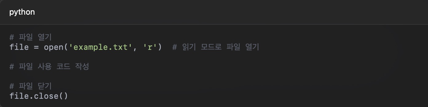
Prior to developing the chatbot, when using tokenizer in CoreML, there is a problem that it cannot be converted from the existing Python code.

CoreML has a problem because it receives a "number array" as input, and the "string" input cannot be converted. When converting a PyTorch or TensorFlow model to Core ML, only the weight and operation of the model are converted, and the tokenizer operates in Python code, so it is deleted without being converted.

Therefore, a temporary model was implemented to confirm whether the function of the kobert model was executed when converting the KoBERT model to the CoreML model.

Methods for converting the Kobert model into the CoreML model is as follow.

• Initial Implementation Method : PyTorch → ONNX → CoreML

Why convert the pytorch model through ONNX instead of directly converting it to CoreML? 

-> Because Open Neural Network Exchange (ONNX) translates models into intermediate formats, increasing compatibility across different frameworks!
Core ML does not fully support the direct transformation of PyTorch models, so it can be transformed more reliably through ONNX.

PyTorch → ONNX → CoreML

[PyTorch Model] → (ONNX Converting) → [ONNX Model] → (CoreML Converting) → [CoreML Model],
Run the Core ML model on iOS

Since mlmodel cannot be opened in Xcode, it is recommended to change it to mlpackage format and open it in an ios environment. In addition, when opening a file converted from Xcode, you should check whether the input and output sizes and types are the same. When the file was opened in Xcode, it was confirmed that int32, the data type of the input and output of the file, was not converted correctly. Since CoreML does not support int64 or int32, it unifies the input and output types as float32.

When the model of the project is completed in the future, it will be converted into CoreML in the same way as above.

Additionally, when I tried to open mlpackage through Xcode in an ios environment(iMAC 24), an outputSchema problem occurred. 

The cause of the problem was that Bert_model's path was inaccurate.

I learned that it is necessary to double-check the code after changing the name of the folder or moving the data.

Project Overview

This project aims to create a chatbot that analyzes the user's emotions and conveys empathy and comfort in the way the other person wants. Analysis of the user's emotions is analyzed in two ways: text analysis and facial images analysis. Analysis through text aims not only to capture words representing specific emotions, but to infer the user's emotions by grasping the context. In addition, the method of treating according to emotions allows users to respond in the way they want, such as friends, parents, and lovers.

Key Features

- Text-based emotional analysis: It analyzes emotions by analyzing text input by the user. 

- Image-based emotional analysis: analyze the facial image image image that the user posted by analyzing the facial image. 

- Provides response to customized comfort: Based on the analyzed emotions, the user responds with the desired type (EX/parents, friends, lovers, etc.).
- Personal custom: Continuous conversation analyzes minor patterns in individual texts, images, etc. to derive more sophisticated responses.

Model Implementation

The text recognition model and the image recognition model are distinguished and implemented respectively. In the initial plan, the text dataset and the image dataset were combined to be implemented as a single dataset, but due to the problem of data size mismatch, the model that recognizes text and images at the same time was not immediately implemented, but after implementing the text recognition model and the image recognition model respectively, it was decided to create a recognition model by combining them.

The text recognition model implements NLP (natural language processing), especially after analyzing the morpheme of Korean, grasping the context, and inferring emotions. 

KoNLpy is used for Korean morpheme analysis.
In the preprocessing process, the dataset is divided into training, validation, and test sets and calculated at a ratio of 8:1:1.
The training text dataset, which has been preprocessed through NLP, is applied to the LSTM model to proceed with training, and tested with the test text dataset, which is tested 20 times with epoch=20 and the performance of the model is gradually improved. The performance of the model is judged based on Accuracy.  
The performance of the model is aimed at Accuracy Score 0.90 or higher, and if the baseline score is not met, the model is gradually improved through hyperparameter tuning.

The image recognition model is largely divided into a training set and a test set in the entire dataset, and 80% is trained and 20% is prepared as a verification set in the training set. Each training, verification, and test set are calculated at a ratio of 3.2:0.8:1. Each prepared dataset was preprocessed through data augmentation and normalization. 
The preprocessed data is applied to the EfficientNetB0 model to proceed with training, and the test is performed with a test image dataset, and the performance of the model is gradually improved by testing it 20 times with epoch=20. The performance of the model is judged based on Accuracy.

Combining the two completed models, we implement one recognition model and test it in CoreML by adding other features.

Technical stack and development environment

Programming Language: Python

Text Emotion Analysis Model: KoBERT (Korean BERT) (Context-based Emotion Analysis), LSTM + Word2Vec (Current Neural Network for Emotion Analysis)

Image Emotion Analysis Models: CNN (Face Emotion Analysis), EfficientNet (Face Emotion Prediction)

Text Dataset : aihub Emotional Conversation Dataset

https://aihub.or.kr/aihubdata/data/dwld.do?currMenu=&topMenu=&dataSetSn=270&beforeSn=274&inqrySeCode=&intrstDataAt=N&reloadYn=N&useAt=

Image Dataset: FER2013 (Face expression dataset)
https://www.kaggle.com/datasets/msambare/fer2013

Data processing: Numpy (multidimensional array and numerical operations, optimization of vector operations of emotion analysis results), Pandas (storage and analysis of emotion analysis results in data frame format, emotion analysis evaluation and statistics processing), Tensorflow (training and optimization of text emotion analysis models, building CNN models for image emotion analysis)

Development Tools: Jupiter Notebook

Expectation Effectiveness

It provides customized comfort services through emotion analysis and can be used for various services dealing with emotions (psychological counseling, etc.).

After completing the data preprocessing, I will now document the architecture of the model I built.

model overview

The model used for text-based emotion classification follows a CNN + BiLSTM + Attention architecture.

This structure was chosen because it captures not only the sequential characteristics of a sentence but also local patterns, making it well-suited for emotion analysis.

• CNN (Convolutional Neural Network)
  • The Conv1D layer is used to extract local features by capturing consecutive word patterns in a sentence—essentially n-gram information, such as emotion-related expressions that appear in groups of 2 to 3 words.
  • By setting the kernel size to 3 (kernel_size=3), the model is trained to detect patterns at the 3-gram level.
• BiLSTM (Bidirectional Long Short-Term Memory)
  • A bidirectional LSTM is used to capture both the forward and backward context of a sentence.
  • With return_sequences=True, the output at each time step is preserved and passed to the next layer, allowing the Attention mechanism to make use of the full sequence information.
• Attention Layer 
  • This is not a built-in Keras layer, but a custom Attention layer that I implemented myself.
  • It learns attention weights based on the word vectors at each time step and generates a context vector that focuses on the most important parts of the sentence.
  • Internally, it uses two Dense layers (W and V) to compute attention scores, which are then normalized using a softmax function.
  • When a mask is provided, extremely small values are assigned to the padding positions to prevent the model from attending to them.

With this combination, I aimed to enhance emotion classification performance, especially for Korean—a language with a flexible word order.

model implementation and design

The model was implemented using TensorFlow and Keras.

The model was trained with the following configuration:

• Loss Function: Sparse Categorical Crossentropy (well-suited for integer-encoded labels)
• Optimizer: Adam (Learning_rate = 0.0003)
• Batch Size: 64
• Epochs: 50
• EarlyStopping & ReduceLROnPlateau : prevent overfitting during training

In addition, to address class imbalance in the dataset, class_weight was used to assign appropriate weights during training.

An ensemble approach was also applied, selecting the best-performing model based on validation accuracy.

Detailed training parameters and performance results will be covered in the next post.

Lessons Learned from Building a Text Classification Model

Designing and implementing the model architecture was a process filled with important decisions and challenges.

One of the biggest difficulties was balancing model complexity with training stability—especially when combining convolutional and recurrent layers with a custom attention mechanism.

It required careful experimentation to ensure that each layer added meaningful value without introducing unnecessary overhead.

In particular, handling the flexible word order of the Korean language posed unique modeling challenges, which led me to choose a BiLSTM + Attention structure that could dynamically capture both local and contextual features.

Through this experience, I realized how crucial it is to design models not only for accuracy, but also for robustness, scalability, and relevance to the linguistic structure of the target domain—principles that are essential in any real-world AI application.

article overview

During the chatbot development process, I will write on the topic of the text data preprocessing process.

I will mainly describe the pre-processing process and what I learned, errors, and what I learned in the process.

development process

Pre-processing is the process of loading a dataset and making it available for model training.

I selected KOTE as the dataset to be used for model training, and the data is stored in .tsv format.

Furthermore, since chatbot development is a multimodal project and will also cover image processing, we have integrated KOTE's 44 emotion labels into seven to fit the labels of Fer2013 - a dataset used for image processing. 

The reason for doing this is to prevent the labels from mixing when combining the models in the last final model, so that the correct response is generated.

First, I will load and save the KOTE dataset. And mapping was conducted to organize emotions into 7 labels.

Tokenization is performed in morpheme units, and I used Mekab to tokenize.

In order for the model to better learn the core content (emotional analogy) of the text, it was intended to exclude unnecessary elements for emotional inference as much as possible.
Words that appear frequently in the text, but have no meaning in emotional analysis, were designated and removed as stopwords.

And because the KOTE dataset is based on online comments, custom tokens have been created so that the model can learn correctly about new words(internet slang) that may not be familiar. 
Integer encoding and padding are performed to convert text data into numbers, and padding is performed to match the input length equally.

Finally, the preprocessing process is completed when the data to be used for model training is converted into an array form and prepared.

errors (Difficulties faced while working on the project)

I thought about how to deal with labels if multiple emotions appear in a single sentence.

For multiple emotions (label strings) in the KOTE dataset, I selected only one main emotion that appeared the most (based on FER2013) and converted it into a single label.

Due to the version compatibility of Mecab and tensorflow and errors in the keras and macOS environments, it was very difficult to import Mecab.

The default path was not recognized, which caused a loading failure. To resolve this, the environment variable MECABRC was manually set, and the dicpath was explicitly specified when initializing the Mecab instance.

In addition, the proportion of OOV (Out-of-Vocabulary) tokens in the dataset was relatively high, introducing noise that interfered with meaningful learning.

To address this issue, the previously limited MAX_VOCAB_SIZE was adjusted based on the number of words learned by the Tokenizer (word_index).

This allowed for a broader vocabulary coverage and significantly reduced the OOV rate.

Challenges and Insights in preprocessing experience

Text data preprocessing is a crucial step for improving both model performance and learning efficiency.

At first, I only had a basic understanding of preprocessing and thought it was important in theory — but I didn’t truly grasp how critical it was in practice.

Because I proceeded with the complacent assumption that “this should be enough,” I didn’t realize the real impact of preprocessing until I reached the model evaluation and performance tuning stages.

I realized that the performance of a model can vary significantly depending on how well the data has been preprocessed. It’s important to thoroughly prepare the data in advance — ensuring that it fits the model architecture and is free of noise.

In this article, we will discuss ways to modify data frames.

Adding columns to a DataFrame

We might want to add new information or perform a calculation based on the data that we already have.

We want to add a column to an existing DataFrame.

Suppose we own a hardware store called The Handy Woman and have a DataFrame containing inventory information:

One way that we can add a new column is by giving a list of the same length as the existing DataFrame.

We can also add a new column that is the same for all rows in the DataFrame.

Finally, we can add a new column by performing a function on the existing columns.

Often, the column that we want to add is related to existing columns.

We can use the apply function to apply a function to every value in a particular column.

For example, this code overwrites the existing 'Name' columns by applying the function upper to every row in 'Name':

df['Name'] = df.Name.apply(str.upper)

In Pandas, we often use lambda functions to perform complex operations on columns.

We can also operate on multiple columns at once.

If we use apply without specifying a single column and add the argument axis=1, the input to our lambda function will be an entire row, not a column.

To access particular values of the row, we use the syntax row.column_name or row[‘column_name’].

Suppose we have a table representing a grocery list:

If we want to add in the price with tax for each line, we’ll need to look at two columns: Price and Is taxed?.

If Is taxed? is Yes, then we’ll want to multiply Price by 1.075 (for 7.5% sales tax).

If Is taxed? is No, we’ll just have Price without multiplying it.

Renaming columns

When we get our data from other sources, we often want to change the column names.

We can change all of the column names at once by setting the .columns property to a different list.

This command edits the existing DataFrame df.

You also can rename individual columns by using the .rename method.

The code above will rename name to First Name and age to Age.

Using rename with only the columns keyword will create a new DataFrame, leaving your original DataFrame unchanged. That’s why we also passed in the keyword argument inplace=True.

Using inplace=True lets us edit the original DataFrame.

There are several reasons why .rename is preferable to .columns:

• You can rename just one column
• You can be specific about which column names are getting changed (with .column you can accidentally switch column names if you’re not careful)

Introducing Pandas 

Pandas is a tool for processing data, that is, a module for processing data by converting various types of data into data frames with rows and columns. For example, converting CSV files or SQL databases into tables.

Converted data frames are organized like tables or spreadsheets. Both rows and columns have indexes, and we can perform tasks individually on rows or columns.

Pandas has the advantage of being able to easily change and manipulate data, which has useful functions for processing missing data, performing tasks on columns and rows, and converting data.

Creating Data with Pandas

In order to get access to the Pandas module, we’ll need to install the module and then import it into a Python file.

After importing Pandas under the name pd easily, what we will do is to turn the data into a data frame format.

DataFrames have rows and columns. Each column has a name, which is a string. Each row has an index, which is an integer. DataFrames can contain many different data types: strings, ints, floats, tuples, etc.

You can pass in a dictionary to pd.DataFrame().

Each key is a column name and each value is a list of column values. The columns must all be the same length or we will get an error.

The above command is an example of creating a data frame, and the resulting df1 is as follows.

Alternatively, there is a method of making columns separately as follows without using a dictionary.

Now we know how to make a data frame.
In this way, we can create our own data frames, but in most cases we will work with large datasets that already exist.
One of the most common forms is the Common Seperated Values (CSV).

Loading Data with Pandas

CSV (comma separated values) is a text-only spreadsheet format.

The first row of a CSV contains column headings. All subsequent rows contain values. Each column heading and each variable is separated by a comma:

When we have data in a CSV, you can load it into a Dataframe in Pandas using .read_csv():

In the example above, the .read_csv() method is called. The CSV file called my-csv-file is passed in as an argument. 

We can also save data to a CSV, using .to_csv():

when we load a new DataFrame from a CSV, we want to know what it looks like.

If it’s a small DataFrame, you can display it by typing print(df).

If it’s a larger DataFrame, it’s helpful to be able to inspect a few items without having to look at the entire DataFrame.

The method .head() gives the first 5 rows of a DataFrame. If you want to see more rows, you can pass in the positional argument n.

The method df.info() gives some statistics for each column.

Selecting Data with Pandas

Now we know how to create and load data. 

Let’s select parts of those datasets that are interesting or important to our analyses.

Suppose we have the DataFrame called customers, which contains the ages of your customers:

There are two possible syntaxes for selecting all values from a column:

1. Select the column as if we were selecting a value from a dictionary using a key. In our example, we would type customers['age'] to select the ages.
2. If the name of a column follows all of the rules for a variable name (doesn’t start with a number, doesn’t contain spaces or special characters, etc.), then we can select it using the following notation: df.MySecondColumn. In our example, we would type customers.age.

When we have a larger DataFrame, we might want to select just a few columns.

To select two or more columns from a DataFrame, we use a list of the column names. 

 new_df = orders[['instance_one', 'instance_two']]

If you want to select a particular row rather than a column, use the iloc[] method.

orders.iloc[2] : It refers to the third row of the order data frame.

we can also select multiple rows from a DataFrame.

Here are some different ways of selecting multiple rows:

• orders.iloc[3:7] would select all rows starting at the 3rd row and up to but not including the 7th row (i.e., the 3rd row, 4th row, 5th row, and 6th row)
• orders.iloc[:4] would select all rows up to, but not including the 4th row (i.e., the 0th, 1st, 2nd, and 3rd rows)
• orders.iloc[-3:] would select the rows starting at the 3rd to last row and up to and including the final row

You can select a subset of a DataFrame by using logical statements:

df[df.MyColumnName == desired_column_value]

Suppose we want to select all rows where the customer’s age is 30. We would use:

df[df.name == 30]

We can also use other logical statements in the same way and combine multiple logical statements, as long as each statement is in parentheses.

For instance, suppose we wanted to select all rows where the customer’s age was under 30 or the customer’s name was “Martha Jones”:

df[(df.age < 30) | df.name == 'Martha Jones')]

Suppose we want to select the rows where the customer’s name is either “Martha Jones”, “Rose Tyler” or “Amy Pond”.

We can use the isin command to check that df.name is one of a list of values:

df[df.name.isin(['Martha Jones', 'Rose Tyler', 'Amy Pond'])]

When we select a subset of a DataFrame using logic, we end up with non-consecutive indices. 

This makes it hard to use .iloc().

We can fix this using the method .reset_index(). For example, here is a DataFrame called df with non-consecutive indices:

If we use the command df.reset_index(), we get a new DataFrame with a new set of indices:

Note that the old indices have been moved into a new column called 'index'. Unless you need those values for something special, it’s probably better to use the keyword drop=True so that you don’t end up with that extra column. If we run the command df.reset_index(drop=True), we get a new DataFrame that looks like this:

Using .reset_index() will return a new DataFrame, but we usually just want to modify our existing DataFrame. If we use the keyword inplace=True we can just modify our existing DataFrame.

df.reset_index(drop=True, inplace=True)

It helps voiding the creation of a new DataFrame and thus improbing memory efficiency.

Before evaluating the performance with the test dataset, we first judged whether the model was overfitting through two training sessions.

When trained with training and validation datasets in the first model, Performance of Accuracy = 0.8257 and val_accuracy = 0.5418. 

When trained with training and validation datasets in the second model, The performance of Accuracy = 0.9244, val_accuracy = 0.3894 was shown.

As we learned more, the accuracy of the training set increased and the accuracy of the verification set decreased This suggests that the model is overfitting the training data. 

Data preprocessing and hyperparameter tuning were modified to prevent overfitting of the model and increase the accuracy of the test set.

The learning rate and dropout figures were considered.However, the epoch was set at the same time as 50, early stopping and call back.  

1. Modifying the list of unused terminology

In the process of tokenizing text data, unnecessary words are removed through a list of terminology, allowing the model to infer emotions from the text more effectively.

Before editing: [‘은', '는', '이', '가', '을', '를']

After modification: [ "의", "가", "이", "은", "들", "는", "좀", "잘", "걍", "과", "도", "를", "으로", "자", "에", "와", "한", "하다", "에서", "까지", "부터", "마다", "보다", "더", "만", "요", "그리고", "그러나", "하지만", "또한", "때문에", "그래서", "무엇", "어디", "왜", "어떻게", "그래도", "그런데", "그러면", "하면", "이다", "이런", "저런", "뿐", "만큼", "정도" ]

The terminology was mainly composed of investigations, connection words, and verbs that did not contain meaning in the word itself. 

Since the text recognition model is made possible to grasp the context of sentences using a hybrid model combining CNN and Bi-LSTM, conjunctions that can infer the context are excluded from the list. 

As a result, the accuracy of the test set increased from 0.5670 (before modification) to 0.5907 (after modification).

2. Modify Dropout

Although the test set's accuracy rose to 0.5907 with a slight modification to the non-verbal list, we were still concerned about the possibility of overfitting considering that the training set is still high and the verification and test sets are low.

Therefore, the number and value of dropout layers were considered as a solution.

Among the number and figures of dropout layers, it was questioned which factors were more influential in preventing overfitting, and to find out, the degree of overfitting was determined by modifying the value of the dropout from 0.4 to 0.5 instead of reducing the dropout by one in the existing model.

Before modificaton: 0.5907

After modification (down by 1 Dropout layer, up to 0.5 Dropout value): 0.6162

When comparing the pre-correction accuracy with the post-correction accuracy, The accuracy of the training set decreased, the accuracy of the verification set increased, and the accuracy of the test set also increased.

From this, it may vary depending on the situation of each model, but in the current model, it was found that the number of dropout layers has a greater impact on overfitting prevention.

3. Modifying the Learning Rate

Existing Learning Rate : 0.0001

Test accuracy when learning rate is 0.0003: 0.6162 -> 0.6212

Test accuracy when learning rate is 0.0005: 0.6212 -> 0.6104

Test accuracy when learning rate is 0.001: 0.6104 -> 0.6152

When the number increased from the existing learning rate of 0.0001 to 0.0003, the test accuracy increased After that, even if the learning rate increased, there was little difference in accuracy.Through this, the model was trained assuming an optimal learning rate of 0.0003.

Python에서 파일 처리는 데이터를 영구적으로 저장하고 읽어오는 데 필수적인 기능입니다. 이번 포스팅에서는 파일을 여는 방법부터 읽기, 쓰기, 닫기, 그리고 다양한 파일 형식(CSV, JSON) 처리까지 자세히 알아보겠습니다.

1. 파일 열기와 닫기 

파일을 사용하려면 먼저 open() 함수를 통해 열어야 합니다. 파일을 다 사용한 후에는 close() 메서드로 닫아주는 것이 좋습니다.

그러나 파일을 열고 닫는 과정에서 예외가 발생할 수 있으므로, with 문을 사용하면 자동으로 파일을 닫아주어 안전합니다.

2. 파일 모드

open() 함수는 두 번째 인자로 파일 모드를 받습니다. 주요 모드는 다음과 같습니다:

• 'r': 읽기 모드 (파일이 존재해야 함)

• 'w': 쓰기 모드 (파일이 없으면 생성, 있으면 내용 삭제)

• 'a': 추가 모드 (파일이 없으면 생성, 있으면 내용 끝에 추가)

• 'b': 바이너리 모드 (예: 'rb', 'wb')

• 바이너리 모드

Python에서 open() 함수의 모드에 'b'를 추가하면 파일이 바이너리 모드로 열립니다.

바이너리 모드는 데이터를 바이트(byte) 단위로 처리하며, 텍스트 인코딩/디코딩 과정 없이 파일의 원본 데이터 그대로를 읽거나 쓸 수 있습니다.

사용 이유

• 텍스트 파일이 아닌 이미지, 오디오, 동영상, 실행 파일 등을 처리할 때.

• 데이터의 원본 상태를 유지하며 읽고 써야 할 때.

• 텍스트가 아닌 데이터는 일반적인 텍스트 모드('r', 'w')로 처리하면 깨질 수 있습니다.

바이너리 모드와 주요 파일 모드의 조합

바이너리 모드 사용 시 주의사항

1. 텍스트와 바이너리 데이터 구분

    • 데이터가 바이트 객체(bytes)로 반환됩니다. 텍스트 데이터를 처리하려면 디코딩(decode)이 필요합니 다.

2. 텍스트 모드와의 차이점

    • 텍스트 모드는 문자열(str)로 데이터를 읽고 쓰며, 자동으로 인코딩/디코딩을 처리합니다.

    • 바이너리 모드는 바이트(bytes) 단위로 데이터를 처리하며, 인코딩/디코딩을 하지 않습니다.

3. 플랫폼 간 차이점

    • 텍스트 모드에서는 파일의 개행 문자(\n)가 운영 체제에 따라 변환됩니다. 바이너리 모드는 변환 없이 데이터를 그대로 처리합니다.

4. 파일 크기 확인

    • 바이너리 모드를 사용할 때는 파일 크기를 확인하거나 특정 바이트를 처리하는 데 유용합니다.

바이너리 모드가 사용되는 주요 사례

1. 이미지 및 동영상 처리:

    바이너리 데이터를 읽고 써서 이미지 파일을 복사하거나 동영상 데이터를 처리.

2. 파일 전송 및 소켓 프로그래밍:

    네트워크 프로토콜에서 파일 데이터를 바이트 단위로 전송.

3. 파일 암호화 및 압축:

    데이터의 원본 상태를 유지하면서 암호화하거나 압축 작업 수행.

3. 파일 읽기 : Reading a file

1) 전체 내용 읽기

 read() 메서드를 사용하여 파일의 전체 내용을 읽을 수 있습니다.

2) 한 줄씩 읽기

 readline() 메서드는 한 번 호출에 한 줄씩 읽어옵니다.

3) 모든 줄을 리스트로 읽기

 readlines() 메서드는 파일의 모든 줄을 리스트로 반환합니다.

4. 파일 쓰기 : Writing a file

1) 새 파일에 쓰기

쓰기 모드 'w'를 사용하면 파일에 데이터를 쓸 수 있습니다. 파일이 이미 존재하면 기존 내용을 삭제하고 새로 작성합니다.

2) 파일에 내용 추가하기

추가 모드 'a'를 사용하면 기존 내용에 새로운 내용을 덧붙일 수 있습니다.

5. 파일 위치 제어

파일 객체는 현재 읽기/쓰기 위치를 기억합니다. tell() 메서드로 현재 위치를 확인하고, seek() 메서드로 위치를 변경할 수 있습니다.

6. 다양한 파일 형식 다루기

1) CSV 파일

CSV(Comma-Separated Values) 파일은 데이터 저장에 널리 사용됩니다. Python의 csv 모듈을 사용하여 CSV 파일을 읽고 쓸 수 있  습니다.

2) JSON 파일

JSON(JavaScript Object Notation) 파일은 데이터 교환에 자주 사용됩니다. Python의 json 모듈을 사용하여 JSON 데이터를 파싱하고 생성할 수 있습니다.

7. 파일 처리 시 주의사항

• 파일 닫기:

   with 문을 사용하여 파일을 자동으로 닫도록 하면 안전합니다. 파일을 직접 닫지 않아도 되므로 예외 상황에서도 자원을 효율적으로 관리     할 수 있습니다.

• 예외 처리:

   파일 작업 중 예외가 발생할 가능성이 있으므로, try…except 블록을 사용하여 오류를 처리하세요.

• 파일 모드 확인:

   파일 작업 전 올바른 모드를 선택하여 데이터 손실을 방지하세요. 예를 들어, 'w' 모드는 기존 내용을 삭제하고 새로 작성하므로 주의가 필     요합니다.

Python의 파일 처리는 데이터를 읽고 쓰는 기본적인 작업부터, CSV, JSON과 같은 구조화된 파일 형식의 처리까지 다양한 작업을 지원합니다. 파일 처리에서 중요한 점은 올바른 파일 모드의 선택과 예외 상황 관리입니다. 이상으로 포스팅 마치겠습니다.

Python의 딕셔너리(Dictionary)는 데이터를 키(key)와 값(value) 쌍으로 저장하는 자료형입니다. 딕셔너리는 데이터 검색, 수정, 추가, 삭제가 빠르고 간단하게 이루어질 수 있도록 설계된 자료구조로, Python 프로그래밍에서 매우 자주 사용됩니다.

0. 딕셔너리 : Dictionary

딕셔너리는 중괄호 {}를 사용하여 생성하며, 각 요소는 키와 값으로 구성됩니다.

키는 고유해야 하며, 불변 객체만 사용할 수 있습니다. 값은 모든 데이터 타입이 가능합니다.

• 키(key): 고유하며 불변 객체(문자열, 숫자, 튜플 등)만 사용 가능. 가변객체(리스트, 딕셔너리)는 사용 불가능.

• 값(value): 모든 데이터 타입 사용 가능하며, 중복 허용.

딕셔너리의 주요 특징

1. 키-값 쌍 저장: 각 키는 고유하며, 이를 통해 데이터를 효율적으로 검색할 수 있습니다.

2. 순서 보장: Python 3.7부터 딕셔너리는 삽입 순서를 유지합니다.

3. 가변성: 딕셔너리는 생성 후에도 수정, 추가, 삭제가 가능합니다.

4. 효율성: 키를 사용한 데이터 검색 속도가 빠릅니다.

1. 딕셔너리 생성 방법

1.1 기본 생성

1.2 dict() 함수 사용

1.3 빈 딕셔너리 생성

2. 딕셔너리의 키(key)와 값(value) 자세히 알아보기

1) 키(key)의 특징

• 불변 객체만 사용 가능: 문자열, 숫자, 튜플 사용 가능.

• 고유성: 딕셔너리에서 동일한 키가 여러 번 지정되면 마지막 값만 유지됩니다.

2) 값(value)의 특징

• 모든 데이터 타입 허용: 값으로 리스트, 딕셔너리 등 가변 객체도 가능.

• 중복 허용: 값은 중복될 수 있으며, 동일한 값을 여러 키에 연결 가능.

3) 키와 값의 관계

• 딕셔너리는 키를 사용하여 값을 빠르게 검색할 수 있는 데이터 구조.

• 키 존재 여부는 in 연산자를 사용해 확인 가능.

3. 딕셔너리 주요 메서드와 활용

1) 값 추가 및 수정

2) 값 삭제

• pop(key): 지정한 키-값 삭제.

• popitem(): 마지막으로 추가된 키-값 삭제.

3) 키가 존재하지 않을 경우 기본값 반환

• get(key, default): 키가 없을 경우 기본값 반환.

4) 딕셔너리 병합

• update(): 다른 딕셔너리의 키-값 추가 또는 업데이트.

5) 딕셔너리 키와 값 추출

• keys(), values(), items() 사용.

4. 딕셔너리 컴프리헨션 : Dictionary Comprihension

딕셔너리 컴프리헨션을 사용하면 간단한 조건이나 규칙에 따라 딕셔너리를 생성할 수 있습니다.

5. 딕셔너리 순회

1) 기본 순회

2) 중첩된 딕셔너리 순회

6. 중첩 딕셔너리

Python에서는 딕셔너리 안에 딕셔너리를 값으로 넣을 수 있습니다. 이를 중첩 딕셔너리(Nested Dictionary)라고 합니다. 딕셔너리 내부의 값으로 또 다른 딕셔너리를 사용하면, 복잡한 계층 구조의 데이터를 효율적으로 표현하고 관리할 수 있습니다.

1. 중첩 딕셔너리 생성

key값으로는 가질 수 없습니다. 반드시 value 값으로 가져야합니다.

2. 중첩 딕셔너리 값 접근

키를 체인 방식으로 접근하여 내부 딕셔너리의 특정 값을 가져올 수 있습니다.

3. 중첩 딕셔너리 값 수정

내부 딕셔너리의 특정 키의 값을 수정할 수 있습니다.

4. 중첩 딕셔너리 값 추가

기존 내부 딕셔너리에 새로운 키-값 쌍을 추가하거나, 외부 딕셔너리에 새로운 내부 딕셔너리를 추가할 수 있습니다.

5. 중첩 딕셔너리 순회

for 루프를 사용하여 중첩 딕셔너리를 순회하면서 키와 값을 처리할 수 있습니다.

출력 결과:

6. 중첩 딕셔너리와 JSON 데이터

중첩 딕셔너리는 JSON(JavaScript Object Notation) 구조와 유사하므로, JSON 데이터를 파이썬 딕셔너리로 쉽게 변환하거나 저장할 수 있습니다.

중첩 딕셔너리 활용 사례

1. 데이터베이스: 사용자 프로필, 상품 카탈로그 등 계층적인 데이터를 저장합니다.

2. 설정 파일: 애플리케이션의 설정 값을 계층적으로 관리합니다.

3. API 응답 처리: REST API의 JSON 응답을 처리합니다.

7. 딕셔너리 사용 시 주의사항

1) 키로 불변 객체만 사용

리스트와 같은 가변 객체는 키로 사용할 수 없습니다. 키로는 문자열, 숫자, 튜플 사용 권장.

2) 중복 키 방지

동일한 키가 여러 번 사용되면 마지막 값만 유지되므로, 중복 키 추가를 방지해야 합니다.

3) 깊은 복사와 얕은 복사

중첩 딕셔너리를 복사할 때는 deepcopy를 사용하여 독립적으로 작업하세요.

4) 키 존재 여부 확인

키가 존재하지 않을 경우 get() 메서드나 in 연산자로 안전하게 접근하세요.

Python 딕셔너리는 데이터를 효율적으로 관리하고 처리할 수 있는 강력한 도구입니다. 다양한 메서드와 활용법을 이해하면 더 유연하고 강력한 프로그램을 작성할 수 있습니다. 이상으로 포스팅 마치겠습니다.

Python에서 문자열(String)은 문자들의 연속으로 구성된 데이터 타입으로, 텍스트 데이터를 처리하는 데 필수적입니다. 이번 포스팅에서는 문자열의 기본 개념과 다양한 문자열 메서드를 활용하는 방법까지 체계적으로 정리해보겠습니다.

0. 문자열 : Strings

문자열은 시퀀스 데이터 타입으로, 각 문자는 고유한 인덱스를 가지며, 다양한 내장 메서드를 사용해 조작할 수 있습니다. 문자열은 불변 객체이므로 직접 수정할 수 없으며, 새로운 문자열을 생성해야 합니다.

Python에서 문자열은 작은따옴표(')나 큰따옴표(")로 감싸서 생성할 수 있습니다.

여러 줄 문자열은 세 개의 작은따옴표(''') 또는 세 개의 큰따옴표(""")로 감쌉니다.

문자열의 특징

• 불변성(Immutability): 문자열은 한 번 생성되면 변경할 수 없습니다.

• 인덱싱(Indexing): 문자열의 각 문자는 인덱스를 통해 접근할 수 있습니다.

• 슬라이싱(Slicing): 문자열의 부분 문자열을 추출할 수 있습니다.

이스케이프 문자 (Escape Characters)

문자열 내에서 특수 문자를 삽입하거나, 줄 바꿈 등의 형식을 표현하기 위해 이스케이프 문자(Escape Characters)를 사용합니다. 이스케이프 문자는 역슬래시(\)와 특정 문자의 조합으로 구성됩니다.

1. 문자열 인덱싱과 슬라이싱

1.1 인덱싱

문자열의 각 문자는 인덱스를 사용해 접근할 수 있습니다.

양수 인덱스는 왼쪽에서 오른쪽으로, 음수 인덱스는 오른쪽에서 왼쪽으로 동작합니다.

1.2 슬라이싱

문자열의 부분 문자열을 추출하려면 슬라이싱을 사용합니다.

구문: string[start:end:step]

2. 문자열 연산

1) 문자열 연결

+ 연산자를 사용해 두 문자열을 연결합니다.

2) 문자열 반복

* 연산자를 사용해 문자열을 반복합니다.

3. 문자열 메서드

Python은 문자열 조작을 위한 다양한 내장 메서드를 제공합니다.

1) 문자열 분할 (Splitting Strings)

 split() 메서드는 문자열을 특정 구분자(separator)로 나누어 리스트로 반환합니다. 구분자를 지정하지 않으면 공백을 기준으로 분리합니   다.

2) 문자열 결합 (Joining Strings)

 join() 메서드는 리스트 등의 이터러블 요소를 하나의 문자열로 결합합니다.

3) 문자열 치환 (Replacing Strings)

 replace() 메서드는 문자열의 특정 부분 문자열을 다른 문자열로 교체합니다.

4) 문자열 검색 (Finding Strings)

 find() 메서드는 특정 부분 문자열이 처음 등장하는 인덱스를 반환하며, 찾지 못하면 -1을 반환합니다.

5) 문자열 포맷팅 (Formatting Strings)

 문자열 포맷팅은 템플릿을 사용해 데이터를 동적으로 문자열에 삽입할 수 있도록 도와줍니다.

 format() 메서드와 f-strings를 사용합니다.

6) 대소문자 변환

• upper(): 문자열을 대문자로 변환.

• lower(): 문자열을 소문자로 변환.

• title(): 각 단어의 첫 문자를 대문자로 변환.

7) 공백 제거

• strip(): 양쪽 공백 제거.

• lstrip(): 왼쪽 공백 제거.

• rstrip(): 오른쪽 공백 제거.

문자열 메서드 비교 요약

4. 문자열 활용 팁

1) 문자열 포함 여부 확인

 in 키워드를 사용해 특정 문자열이 포함되어 있는지 확인할 수 있습니다.

2) 문자열 길이 구하기

 len() 함수로 문자열의 길이를 구할 수 있습니다.

3) 문자열 순회

 for 반복문을 사용하여 문자열의 각 문자를 순회할 수 있습니다.

출력 결과:

5. 문자열 사용 시 주의할 점

1) 불변성: 문자열은 불변 객체이므로 수정이 불가능하며, 변경 작업은 항상 새로운 문자열을 생성합니다.

2) 인덱스 오류: 잘못된 인덱스에 접근하면 IndexError가 발생합니다. 인덱스를 확인하고 사용하세요.

3) 공백 처리: 입력값에서 공백은 의도치 않은 결과를 초래할 수 있으므로 strip()을 사용해 처리하는 것이 좋습니다.

Python 문자열은 텍스트 데이터 처리와 조작에서 필수적인 도구입니다. 주요 메서드와 활용 방법을 숙지하면 더욱 효율적인 코드를 작성할 수 있습니다. 이상으로 포스팅 마치겠습니다.